Data items are described in order to ensure an ideal relationship between the length of the text and meta information per item (the name itself identifies the data item precisely) and at the same time enables their engine processing (issue of coding, admissible characters, etc.)
provides an overview of the original description of variables (data items) used in the case study.
Variable group
Abbr. (chap. in method.)
Name of the variable
Variable - definition (1)
Variable- definition (2)
Variable - source (1)****)
Residence
RES-cso (2.3.7)
Residents (CZSO)
A resident is any person who has lived for a long time in the place where he has his household, or family.
RESIDENCE IN THE DECISIVE MOMENT (26. 3. 2011). The place in which the participant has actually lived in the long term and in which he has his household, or family. A person’s permanent residence is not relevant, neither is the fact that a person spends major part of the week at a different place due to work or studies. Where the place of residence differs from the address in the header, it should be noted as precise as possible.
CZSO
Out-commuting
OUTC-cso (2.3.7)
Out-commuters (CZSO)
Out-commuters include people commuting to work and students commuting to schools
In the analysis of the out-commuting, it is assumed that the out-commuters include not only employees (excluding working students and apprentices) but also students (including the working ones).
CZSO
Out-commuting
NOC-cso (2.3.7)
Non-commuters (CZSO)
Non-commuters are non-working pensioners, people with their own livelihood, homemakers, preschool children, other dependent persons and people with no economic activity established
Non-commuters include: // non-working pensioners (u113-101201) // people with their own livelihood (u113-101301) // homemakers, pre-school children, other dependant persons (u113-101401) // people with no economic activity established(u113-101601)
CZSO
Out-commuting
OUTCW-cso_LAU2 (2.3.2)
Out-commuters to work and schools (CZSO)
Out-commuters to work or schools are people residing within the municipality that leave from the municipality to work or school in another municipality
Out-commuters to work or school (CZSO) are people residing within the municipality that leave from the municipality to work or school in another municipality. Data only include economically active participants who state the exact destination of their out-communing.
CZSO
In-commuting
INCW-cso_LAU2 (2.3.2)
In-commuters to work and schools (CZSO)
In-commuters to work and schools are people that do not reside within the territory of the municipality (residing in other municipality than in the in-commuting target municipality) and terminating their trip (with the in-commuting destination) in the given municipality.
In-commuters to work and schools (CZSO) are people that do not resided within the territory of the municipality (residing in other municipality than in the in-commuting target municipality), and terminating their trip (with the in-commuting destination) in the given municipality. Data only include economically active participants who state the exact destination of their out-communing.
CZSO
Residence
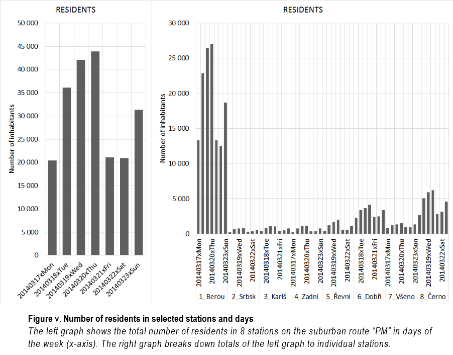
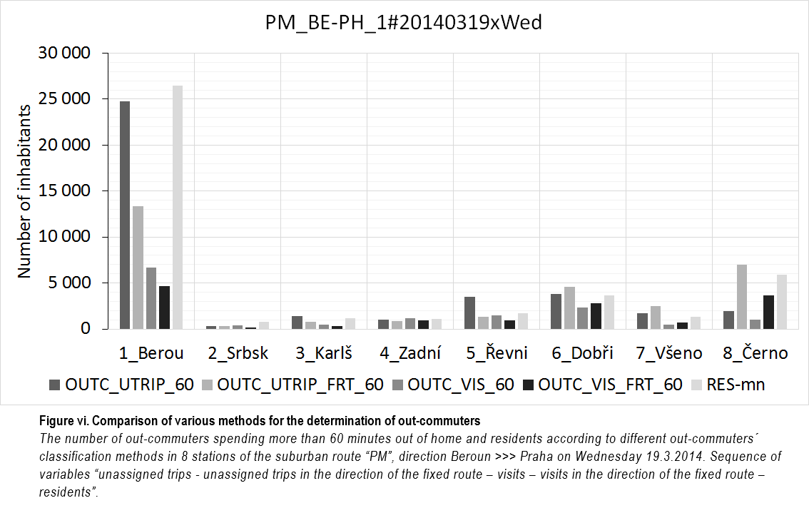
RES-mn (2.3.7)
Residents in the station according to mobile network data
Residents in the station include people who, on the reviewed day, are in the station early in the morning and late in the evening. This station is considered their place of residence.
On a single reviewed day, the participant was recorded in the place early in the morning 0:00:00 - 04:10:00h and in the evening hours 19:50:00 - 23:59:59h
MN
Visits
OUTC_VIS (2.3.2)
Visits of out-commuters residing in the station to destinations outside the station
Visits of out-commuters who left the station of their residence on the reviewed day and spent a defined minimum aggregate time in at least one destination stations. The PLACE OF RESIDENCE-DESTINATION relation.
Visits in destinations are made by the residents of the station who leave the station to arrive in the out-commuting destination in a station other then the station of their residence, and spend a pre-defined period of time within 24 hours (00:00:00 – 23:59:59) in one of the destinations.
MN
Visits
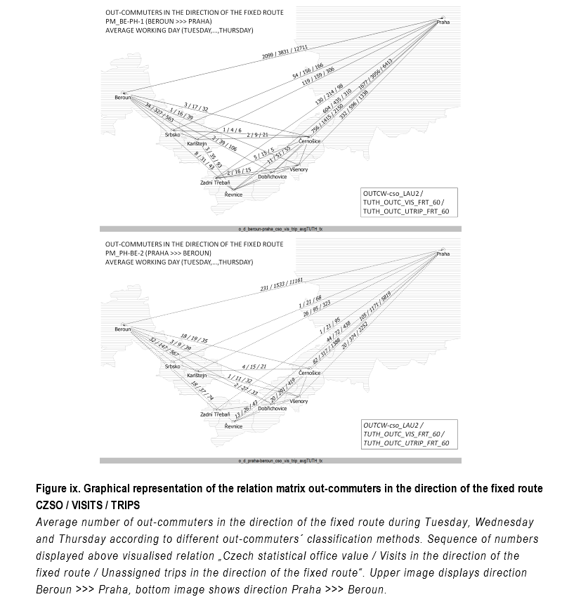
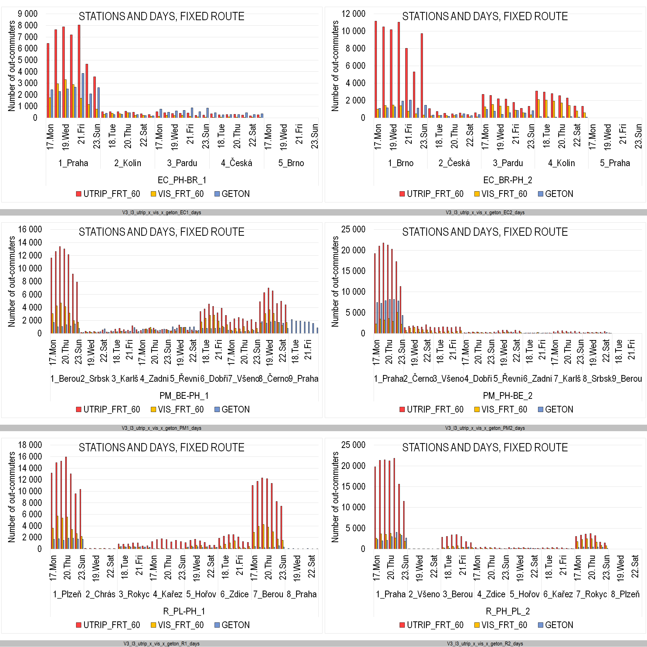
OUTC_VIS_FRT (2.3.2)
Visits of out-commuters residing in the station to destinations outside of the station in the direction of the fixed route.
Visits of out-commuters who left the station of their residence on the reviewed day and spent a defined minimum aggregate time in at least one destination stations in the direction of the fixed route. The PLACE OF RESIDENCE-DESTINATION relation.
Visits in destinations are made by the residents of the station who leave the station to arrive in the out-commuting destination in a station other then the station of their residence, and spend a pre-defined period of time within 24 hours (00:00:00 – 23:59:59) in one of the destinations, provided these stations are located in the direction of the selected fixed route. The relation is established by all stops of the bus or train lines.
MN
Visits
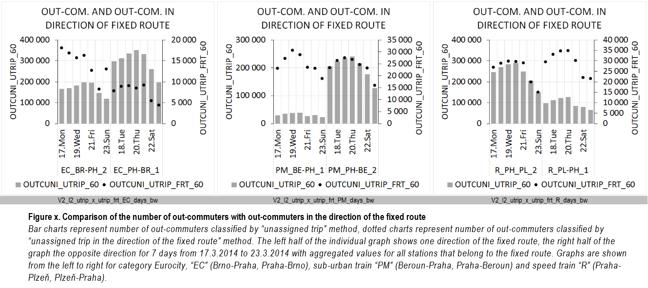
OUTC_UTRIP (2.3.3)
Unlinked passengers´ trips of out-commuting persons who stayed in the station for minimal defined time out of the station
Trips of out-commuting people who left the station on the reviewed day and spent a defined minimum aggregate time in at least one other station within the given day. The SOURCE-DESTINATION relation
Trips into destinations with a defined period of time are made by people in the territory of the station who leave the station for another station in which they spend more than a pre-defined period of time within 24 hours (00:00:00 – 23:59:59).
MN
Visits
OUTC_UTRIP (2.3.3)
Unlinked passengers´ trips of out-commuting persons who stayed in the station for minimal defined time out of the station
Trips of out-commuting people who left the station on the reviewed day and spent a defined minimum aggregate time in at least one other station within the given day. The SOURCE-DESTINATION relation
Trips into destinations with a defined period of time are made by people in the territory of the station who leave the station for another station in which they spend more than a pre-defined period of time within 24 hours (00:00:00 – 23:59:59).
MN
Trips*)
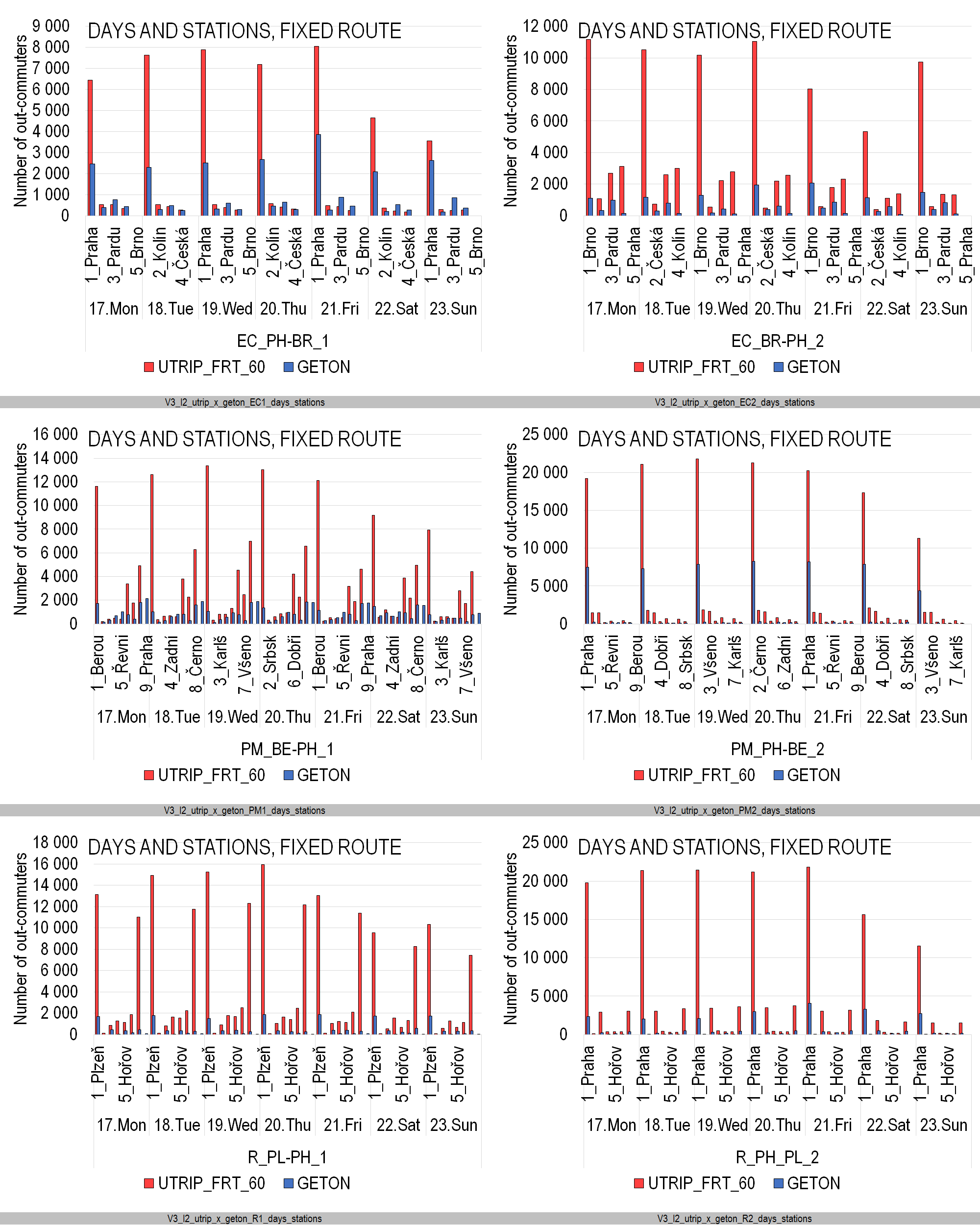
OUTC_UTRIP_FRT (2.3.5)
Unlinked passengers´ trips of out-commuting persons who stayed in the station for minimal defined time out of the station in the direction of the fixed route
Trips of out-commuting people who left the station on the reviewed day and spent a defined minimum aggregate time in at least one other station in the direction of the selected fixed route within the given day. The SOURCE-DESTINATION relation
Trips into destinations with a defined period of time are made by people in the territory of the station who leave the station for another station in the direction of the selected fixed route in which they spend more than a pre-defined period of time within 24 hours (00:00:00 – 23:59:59)
MN
Trips**)
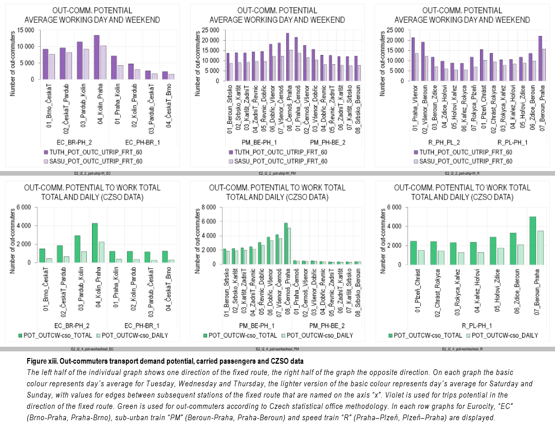
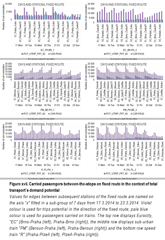
POT_UTRIP_FRT (2.3.6)
Potential of unlinked passengers´ trips who stayed in the station for a minimal defined time out of the station in the direction of the fixed route
Potential of trips of out-commuting people who left the station on the reviewed day and spend a defined minimum aggregate time in at least one different station along the selected fixed route. The ORIGIN-DESTINATION relation
Potential of trips is the sum of trips in the direction of the fixed route with the assumption of the sequence of destinations defined by the fixed route
MN
Trips
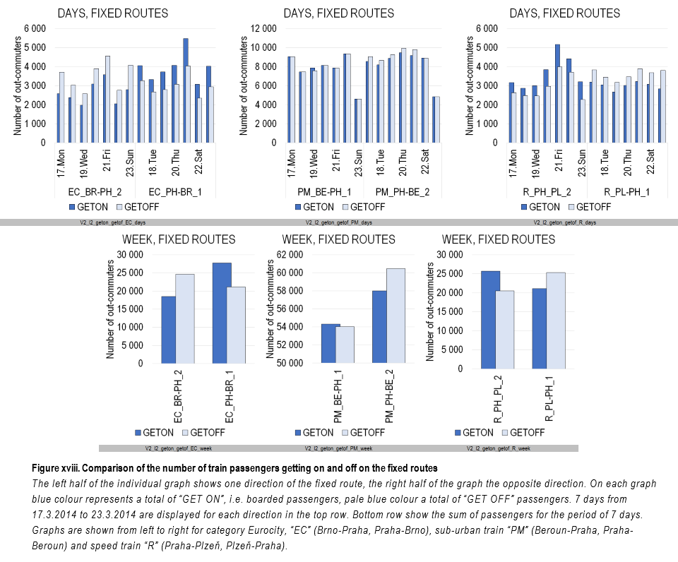
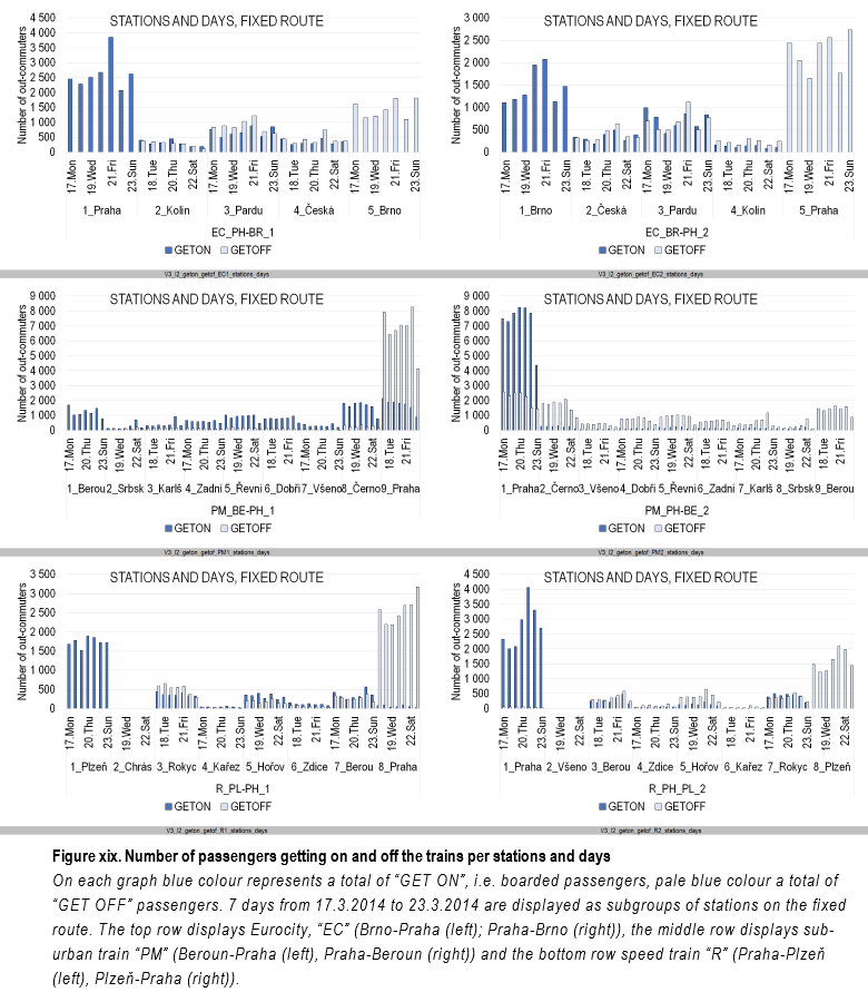
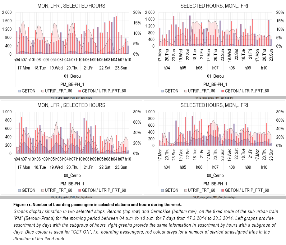
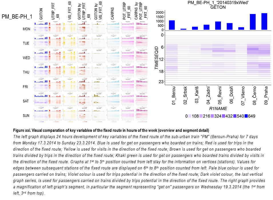
GETON (2.3.7)
Passengers boarding on a train vehicle operating on fixed route of a carrier
Total number of passengers boarding on the reviewed days on the carrier’s train vehicles on a given fixed route in the station and left in the direction of the next station
This includes people that have been ascertained by the counting entity (conductor, train manager) in person in the railway station or in a between-the-stops slot, or established by the mobile network, or by the CHECKIN/OUT system
MN/CAMP
Trips
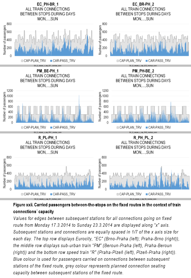
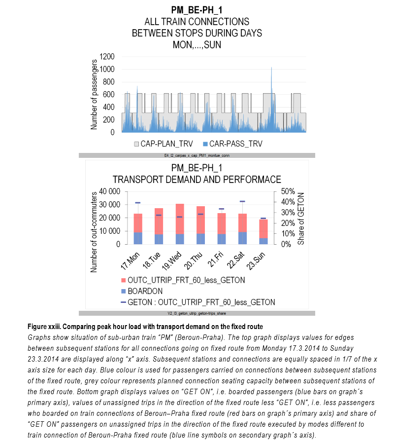
CAP-PL_TRV
The total passenger capacity of a train vehicle operating on a fixed route departing from the stop in the direction of the fixed route(selected day)
Aggregate planned capacity of carrier’s train vehicles set out on the reviewed day from the station into the next station in the direction of the fixed route
Total planned fixed route capacity (seating capacity)
CISJR
Trips***)
CAR-PAS_TRV (2.3.6)
Carried passengers on the train vehicle between stops (occupancy)
Aggregate occupancy of train vehicles between the stops
This includes people that have been ascertained by the counting entity (conductor, train manager) in person in the railway station or in a between-the-stops slot, or established by the mobile network, or by the CHECKIN/OUT system
MN/CAMP
(*) Corresponds to the synthetic indicator ‘PASSENGER TRANSPORT’, see for instance Table 4.
(**) When multiplied by the length of the track stretches, it corresponds to the ‘TRANSPORT PERFORMANCE’ indicator, see for instance. Note: Item does not include trips by people who do not fulfil the definition, i.e. did not stay in the station for more than 60 minutes.
(***) When multiplied by the length of the track stretches it corresponds to the ‘RAIL TRANSPORT PERFORMANCE‘ indicator, see for instance.
(****) CISJR = Nomenclature of public transport flow diagram; MN = mobile network; CAMP = census based campaign; CZSO ´Czech Statistical Office